OpenCV 과제: 영상 색상 채우기 #1

February 20, 2021 8 분 소요

질문

내용

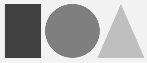
다음 영상 이름은 “hwfig5-1.jpg”이다. 이 영상에 대해 다음을 프로그래밍하시오.

위 영상을 Mat img1 = imread() 함수를 이용하여 grayscale 영상으로 읽어 오시오.
또 다른 영상을 저장하기 위해 Mat img2;로 하고, 이것은 칼라(3채널)로 저장하기 위해 선언하시오.
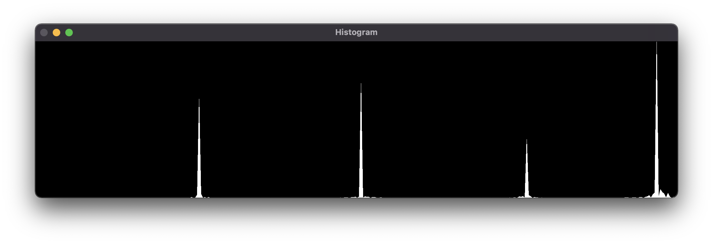
위 영상에 대해 히스토그램을 구하시오.
히스토그램에서 최대 peak가 되는 값 4개를 구하시오. (육안으로…)
각 4개 peak점의 가운데 값을 문턱치로 사용하여 가장 어두운 직사각형은 파랑색, 원은 녹색, 삼각형은 빨강색, 배경은 노랑색으로 하여 img2를 만들어 display하시오.

답변

내용

독자 여러분께서 OpenCV 설치 및 설정을 완료했다는 전제하에 설명을 진행하겠다. (그러므로 아직 설치하지 않았거나 설정하지 않았다면 먼저 이것들을 해결하고 오길 바란다.)

필자가 아마 이 날 캠핑에 갔었던 것으로 기억하고 있는데, 그곳에서 이 과제를 해결해드렸던 기억이 난다.

(과제 마감까지 불과 3시간을 남겨두고;;)

필자가 듣던 바에 의하면 이쪽 학과의 4학년 분들이나 대학원생분들께서 OpenCV와 관련된 공부를 하신다는 것을 알고 있다.

필자는 OpenCV와 관련한 이론을 빠삭히 알고 있지는 못하며, 더군다나 이쪽 학과와는 전혀 관련없는 학과에 재학중인 관계로 이론적인 부분에서 밀리더라도 양해부탁드린다.

(잘못된 내용 잡아서 댓글 남겨주시면 감사드리겠습니다.)

필자는 이 문제를 풀이하기 위해 오로지 직관만 이용하였음을 밝힌다.

암튼 각설하고 풀이를 진행하겠다.

일단 문제에서 시키는 대로 순차적으로 풀이를 진행해주면 된다.

먼저 1번부터 해결해보자.

위 영상을 Mat img1 = imread() 함수를 이용하여 grayscale 영상으로 읽어 오시오.

위에서 언급했던 바와 같이 Mat에 대해서 아는 것이 없어서 인터넷에 검색해봤다.

검색을 통해 Mat는 클래스이고, OpenCV에서 가장 기본이 되는 데이터 타입이며, 행렬 구조체라는 것을 파악할 수 있었다.

또한, imread() 함수에 대해서도 아는것이 없어서 아래의 레퍼런스 문서를 확인해보니

Reference

다음과 같았다.

imread()

Mat cv::imread(const String& filename, int flags = IMREAD_COLOR)

반환형이 위에서 인터넷 검색을 통해 파악했던 Mat이고, 매개변수들의 이름과 기본값을 통해서 첫 번째 인자로는 읽어들이고자 하는 이미지 파일명을, 두 번째 인자로는 색상 채널과 관련된 flags들을 보내주면 된다는 것을 파악하였다.

또한, Mat는 다음의 헤더파일에 선언되어 있고,

#include <opencv2/core/mat.hpp>

imread() 함수는 다음의 헤더파일에 선언되어 있다하니

#include <opencv2/imgcodecs.hpp>

이러한 헤더파일들을 포함시켜주면 되겠다.

그런데 필자는 이러한 과정이 번거로워 opencv2/opencv.hpp 헤더파일만 포함시켰다.

아래에 opencv.hpp의 내용을 보이겠다.

/*M///////////////////////////////////////////////////////////////////////////////////////
//
//  IMPORTANT: READ BEFORE DOWNLOADING, COPYING, INSTALLING OR USING.
//
//  By downloading, copying, installing or using the software you agree to this license.
//  If you do not agree to this license, do not download, install,
//  copy or use the software.
//
//
//                           License Agreement
//                For Open Source Computer Vision Library
//
// Copyright (C) 2000-2008, Intel Corporation, all rights reserved.
// Copyright (C) 2009-2010, Willow Garage Inc., all rights reserved.
// Third party copyrights are property of their respective owners.
//
// Redistribution and use in source and binary forms, with or without modification,
// are permitted provided that the following conditions are met:
//
//   * Redistribution's of source code must retain the above copyright notice,
//     this list of conditions and the following disclaimer.
//
//   * Redistribution's in binary form must reproduce the above copyright notice,
//     this list of conditions and the following disclaimer in the documentation
//     and/or other materials provided with the distribution.
//
//   * The name of the copyright holders may not be used to endorse or promote products
//     derived from this software without specific prior written permission.
//
// This software is provided by the copyright holders and contributors "as is" and
// any express or implied warranties, including, but not limited to, the implied
// warranties of merchantability and fitness for a particular purpose are disclaimed.
// In no event shall the Intel Corporation or contributors be liable for any direct,
// indirect, incidental, special, exemplary, or consequential damages
// (including, but not limited to, procurement of substitute goods or services;
// loss of use, data, or profits; or business interruption) however caused
// and on any theory of liability, whether in contract, strict liability,
// or tort (including negligence or otherwise) arising in any way out of
// the use of this software, even if advised of the possibility of such damage.
//
//M*/

#ifndef OPENCV_ALL_HPP
#define OPENCV_ALL_HPP

// File that defines what modules where included during the build of OpenCV
// These are purely the defines of the correct HAVE_OPENCV_modulename values
#include "opencv2/opencv_modules.hpp"

// Then the list of defines is checked to include the correct headers
// Core library is always included --> without no OpenCV functionality available
#include "opencv2/core.hpp"

// Then the optional modules are checked
#ifdef HAVE_OPENCV_CALIB3D
#include "opencv2/calib3d.hpp"
#endif
#ifdef HAVE_OPENCV_FEATURES2D
#include "opencv2/features2d.hpp"
#endif
#ifdef HAVE_OPENCV_DNN
#include "opencv2/dnn.hpp"
#endif
#ifdef HAVE_OPENCV_FLANN
#include "opencv2/flann.hpp"
#endif
#ifdef HAVE_OPENCV_HIGHGUI
#include "opencv2/highgui.hpp"
#endif
#ifdef HAVE_OPENCV_IMGCODECS
#include "opencv2/imgcodecs.hpp"
#endif
#ifdef HAVE_OPENCV_IMGPROC
#include "opencv2/imgproc.hpp"
#endif
#ifdef HAVE_OPENCV_ML
#include "opencv2/ml.hpp"
#endif
#ifdef HAVE_OPENCV_OBJDETECT
#include "opencv2/objdetect.hpp"
#endif
#ifdef HAVE_OPENCV_PHOTO
#include "opencv2/photo.hpp"
#endif
#ifdef HAVE_OPENCV_STITCHING
#include "opencv2/stitching.hpp"
#endif
#ifdef HAVE_OPENCV_VIDEO
#include "opencv2/video.hpp"
#endif
#ifdef HAVE_OPENCV_VIDEOIO
#include "opencv2/videoio.hpp"
#endif

#endif

이렇듯 opencv.hpp는 대부분 필요한 헤더파일들을 다 포함시켜준다.

그 다음 이미지 파일명과 문제에서 요구한 GrayScale에 해당하는 flag를 인자로 보내주고, 그에 따른 반환값을 img1에 담자.

필자는 아래의 경로에 이미지 파일을 두었다.

/Users/hexk/Desktop/test1.jpg

즉,

Mat img1 = imread("/Users/hexk/Desktop/test1.jpg", IMREAD_GRAYSCALE);

2번도 마찬가지 방식으로 진행하면 된다.

또 다른 영상을 저장하기 위해 Mat img2;로 하고, 이것은 칼라(3채널)로 저장하기 위해 선언하시오.

문제에서 3 Channel Color를 원했으니 그에 해당하는 flag(IMREAD_COLOR)만 인자로 넘겨주자.

즉,

Mat img2 = imread("/Users/hexk/Desktop/test1.jpg", IMREAD_COLOR);

자 이제 대망의 3번이다.

위 영상에 대해 히스토그램을 구하시오.

히스토그램을 그리는 함수를 작성할 차례인데, 필자는 코드의 재사용을 고려하여 함수 draw_Histogram(Return Type: Mat Type, Parameter Type: Mat Reference Type)을 작성했다.

또한, 히스토그램을 그리기 위해 아래의 공식 문서의 예제를 참고했다.

Reference

먼저 히스토그램을 표시할 이미지를 생성하자.

Mat draw_Histogram(Mat& hist) {
    int hist_w = 2048;
    int hist_h = 500;
    int hist_size = 350;
    int bin_w = cvRound((double)hist_w/hist_size);

    Mat histImage(hist_h, hist_w, CV_8UC3, Scalar(0, 0, 0));
}

인자로 받은 hist 값을 normalize하자.

Mat draw_Histogram(Mat& hist) {
    int hist_w = 2048;
    int hist_h = 500;
    int hist_size = 350;
    int bin_w = cvRound((double)hist_w/hist_size);

    Mat histImage(hist_h, hist_w, CV_8UC3, Scalar(0, 0, 0));

    normalize(hist, hist, 0, histImage.rows, NORM_MINMAX, -1, Mat());
}

(필자는 편의를 위해 이름공간인 cv를 사용했다.)

필자는 흰색으로 채워진 볼록 다각형을 그리기 위해 fillConvexPoly Function을 이용했다.

공식 문서에 의하면, fillConvexPoly Function은 다음과 같다.

void cv::fillConvexPoly(InputOutputArray img, 
                        const Point* pts,
                        int npts,
                        const Scalar& color,
                        int lineType = LINE_8,
                        int shift = 0
)

즉, 위에서 생성한 Mat type의 histImage를 첫 번째 인자로 넘겨주고, 점들을 저장한 배열 pts를 두 번째 인자로, 점들의 개수를 세 번째 인자로, 색깔은 Scalar(255, 255, 255)(흰색)를 네 번째 인자로 넘겨주자.

이를 코드로 보이면 다음과 같다.

Mat draw_Histogram(Mat& hist) {
    int hist_w = 2048;
    int hist_h = 500;
    int hist_size = 350;
    int bin_w = cvRound((double)hist_w/hist_size);

    Mat histImage(hist_h, hist_w, CV_8UC3, Scalar(0, 0, 0));

    normalize(hist, hist, 0, histImage.rows, NORM_MINMAX, -1, Mat());

    for(int i=1; i<hist_size; i++) {
        Point pts[] = {Point(bin_w * (i-1), hist_h), Point(bin_w * i, hist_h), Point(bin_w * i, hist_h - cvRound(hist.at<float>(i))), Point(bin_w*(i-1), hist_h-cvRound(hist.at<float>(i-1))), Point(bin_w*(i-1)), hist_h};     // 이렇듯 Point(2차원 점) 객체를 생성하여 Point 배열 pts에 담았다.

        fillConvexPoly(histImage, pts, 5, Scalar(255, 255, 255));
    }
}

이제 히스토그램 확인을 위해 imshow Function을 호출하자.

또한, histImage를 반환하자.

(4번째 문제에서 요구한 바(히스토그램 위에 Peaks를 찍어야 하지 않겠는가?)를 충족시키기 위해)

Mat draw_Histogram(Mat& hist) {
    int hist_w = 2048;
    int hist_h = 500;
    int hist_size = 350;
    int bin_w = cvRound((double)hist_w/hist_size);

    Mat histImage(hist_h, hist_w, CV_8UC3, Scalar(0, 0, 0));

    normalize(hist, hist, 0, histImage.rows, NORM_MINMAX, -1, Mat());

    for(int i=1; i<hist_size; i++) {
        Point pts[] = {Point(bin_w * (i-1), hist_h), Point(bin_w * i, hist_h), Point(bin_w * i, hist_h - cvRound(hist.at<float>(i))), Point(bin_w*(i-1), hist_h-cvRound(hist.at<float>(i-1))), Point(bin_w*(i-1), hist_h)};

        fillConvexPoly(histImage, pts, 5, Scalar(255, 255, 255));
    }

    imshow("Histogram", histImage);

    return histImage;
}

이제 main 함수로 돌아가서 나머지 histogram 설정을 마무리하자.

먼저 histSize를 설정하자.

int main(void) {
    int histSize = 350;

    return 0;
}

그 후 값의 범위도 설정해주자.

int main(void) {
    int histSize = 350;

    float range[] = {0, 256};
    const float* histRange = {range};

    return 0;
}

histSize를 동일한 크기로 만들고 히스토그램을 비우기 위한 bool형 변수도 설정 해주자. (아래에서 calcHist 함수의 인자로 보내줄 예정.)

int main(void) {
    int histSize = 350;

    float range[] = {0, 256};
    const float* histRange = {range};

    bool uniform = true, accumulate = false;

    return 0;
}

마지막으로 히스토그램을 계산하자.

이는 OpenCV 함수 cv::calcHist를 이용하면 된다.

cv::calcHist는 다음과 같으며,

void cv::calcHist(const Mat* images,
                  int nimages,
                  const int* channels,
                  InputArray mask,
                  OutputArray hist,
                  int dims,
                  const int* histSize,
                  const float** ranges,
                  bool uniform = true,
                  bool accumulate = false
)

첫 번째 인자로는 원본 배열(grayscale로 받아들인 img1)을, 두 번째 인자로는 첫 번째 배열의 수(1)를, 세 번째 인자로는 측정될 채널 배열(각 배열은 단일 채널이므로 0)을, 네 번째 인자로는 히스토그램이 저장될 Mat 객체(새로 생성하여 보내주자)를, 다섯 번째 인자로는 히스토그램의 차원(1)을, 여섯 번째 인자로는 histSize(histSize의 주소)를, 일곱 번째 인자로는 각 차원마다 측정될 값들의 범위(histRange의 주소)를, 여덟 번째와 아홉 번째 인자로는 각각 위에서 설정해둔 bool 변수인 uniform과 accumulate를 인자로 보내주면 된다.

즉, 이를 코드로 보이면 다음과 같다.

int main(void) {
    int histSize = 350;

    float range[] = {0, 256};
    const float* histRange = {range};

    bool uniform = true, accumulate = false;

    Mat b_hist;     // 히스토그램이 저장될 Mat 객체 생성

    calcHist(&img1, 1, 0, Mat(), b_hist, 1, &histSize, &histRange, uniform, accumulate);

    return 0;
}

그 후 b_hist 객체를 우리가 위에서 작성한 draw_Histogram 함수의 인자로 보내주면 된다.

(물론 Peaks들을 그려진 히스토그램 위에 그려야 하므로, Mat 객체를 하나 더 생성하여 draw_Histogram의 반환값을 저장하자.)

즉,

int main(void) {
    int histSize = 350;

    float range[] = {0, 256};
    const float* histRange = {range};

    bool uniform true, accumulate = false;

    Mat b_hist;     // 히스토그램이 저장될 Mat 객체 생성
    Mat histImg;    // draw_histogram 반환값을 저장하기 위한 Mat 객체 생성

    calcHist(&img1, 1, 0, Mat(), b_hist, 1, &histSize, &histRange, uniform, accumulate);

    histImg = draw_Histogram(b_hist);

    return 0;
}

마지막으로 잘 출력되는지 확인하기 전에 waitKey() Function도 넣어주자. (이 함수를 호출하지 않으면, 프로그램이 바로 종료되어 히스토그램이 잘 출력되는지 확인할 수 없다.)

int main(void) {
    int histSize = 350;

    float range[] = {0, 256};
    const float* histRange = {range};

    bool uniform true, accumulate = false;

    Mat b_hist;     // 히스토그램이 저장될 Mat 객체 생성
    Mat histImg;    // draw_histogram 반환값을 저장하기 위한 Mat 객체 생성

    calcHist(&img1, 1, 0, Mat(), b_hist, 1, &histSize, &histRange, uniform, accumulate);

    histImg = draw_Histogram(b_hist);

    waitKey();

    return 0;
}

여기까지 했으면 히스토그램은 완성이다.

이제 프로그램을 실행해보자.

아래와 같이 나오면 성공이다.

Result

지금까지 우리가 작성한 전체 코드를 보이면서, 우선 여기에서 한번 끊겠다.

(한 강좌가 너무 길어질 듯하여…)

나머지 문제들은 2편(필요하다면 3편에 걸쳐)에서 풀이하도록 하겠다.

전체 코드

#include <opencv2/opencv.hpp>

using namespace cv;

Mat draw_Histogram(Mat& hist) {
    int hist_w = 2048;
    int hist_h = 500;
    int hist_size = 350;
    int bin_w = cvRound((double)hist_w/hist_size);

    Mat histImage(hist_h, hist_w, CV_8UC3, Scalar(0, 0, 0));

    normalize(hist, hist, 0, histImage.rows, NORM_MINMAX, -1, Mat());

    for(int i=1; i<hist_size; i++) {
        Point pts[] = {Point(bin_w * (i-1), hist_h), Point(bin_w * i, hist_h), Point(bin_w * i, hist_h - cvRound(hist.at<float>(i))), Point(bin_w*(i-1), hist_h-cvRound(hist.at<float>(i-1))), Point(bin_w*(i-1), hist_h)};

        fillConvexPoly(histImage, pts, 5, Scalar(255, 255, 255));
    }

    imshow("Histogram", histImage);

    return histImage;
}

int main(void) {
    int histSize = 350;

    float range[] = {0, 256};
    const float* histRange = {range};

    bool uniform = true, accumulate = false;
    
    Mat img1 = imread("/Users/hexk/Desktop/test1.jpg", IMREAD_GRAYSCALE);
    Mat img2 = imread("/Users/hexk/Desktop/test1.jpg", IMREAD_COLOR);

    Mat b_hist;     // 히스토그램이 저장될 Mat 객체 생성
    Mat histImg;    // draw_histogram 반환값을 저장하기 위한 Mat 객체 생성

    calcHist(&img1, 1, 0, Mat(), b_hist, 1, &histSize, &histRange, uniform, accumulate);

    histImg = draw_Histogram(b_hist);
    
    waitKey(0);

    return 0;
}

Twitter Facebook LinkedIn

Jonghyeok Kim

OpenCV 과제: 영상 색상 채우기 #1

질문

내용

답변

내용

imread()

전체 코드

공유하기

댓글남기기

참고

Capstone Design: 종합설계보고서 및 요약보고서

Notice: 2023년 10월 30일(월) Audio Player 탑재

Exhibition: The Tom Project

Plans: 23.04.23