
Matlab: Tensile Testing
Questions
A tensile testing machine such as the one shown in Figure P5.12(a) and (b) is used to determine the behavior of materials as they are deformed.
Table P5.12 Tensile Testing Data
| Load, lbf | Length, inches |
|---|---|
| 0 | 2.0000 |
| 2000 | 2.0024 |
| 4000 | 2.0047 |
| 6000 | 2.0070 |
| 7500 | 2.0094 |
| 8000 | 2.0128 |
| 8500 | 2.0183 |
| 9000 | 2.0308 |
| 9500 | 2.0500 |
| 10000 | 2.075 |
In the typical test, a specimen is stretched at a steady rate. The force (load) required to deform the material is measured, as is the resulting deformation. An example set of data measured in one such test is shown in Table P5.12. These data can be used to calculate the applied stress and the resulting strain with the following equations.
\[\sigma = \frac{F}{A} \text{ and } \epsilon = \frac{l - l_{0}}{l_{0}}\]where
\[\sigma = \text{ stress in (Psi) } lb_{f}/in.^{2},\] \[F = \text{ applied force in } lb_{f},\] \[A = \text{ sample cross-sectional area in } in.^{2},\] \[\epsilon = \text{ strain in } in./in.,\] \[l = \text{ sample length, and}\] \[l_{0} = \text{ original sample length.}\](a) Use the provided data to calculate the stress and the corresponding strain for each data pair. The tested sample was a rod of diameter $\text{}0.505 in.,$ so you’ll need to find the cross-sectional area to use in your calculations.
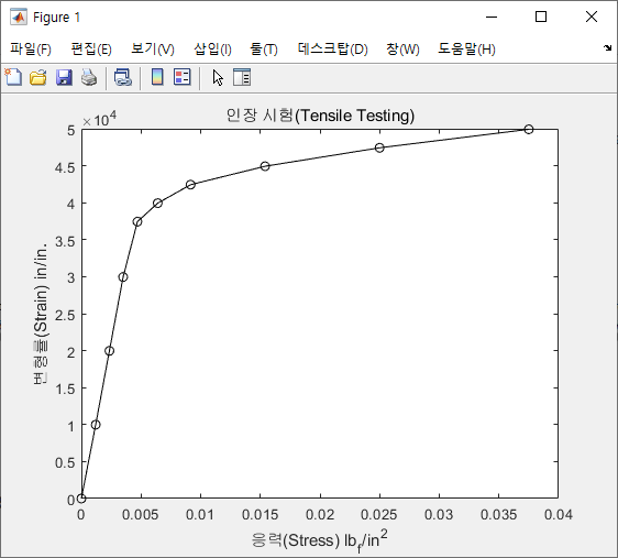
(b) Create an $x-y$ plot with strain on the $x$-axis and stress on the $y$-axis. Connect the data points with a solid black line, and use circles to mark each data point.
(c) Add a title and appropriate axis labels.
(d) The point where the graph changes from a straight line with a steep slope to a flattened curve is called the $\text{yield stress}$ or $\text{yield point}$. This corresponds to a significant change in the material behavior. Before the yield point the material is elastic, returning to its original shape if the load is removed - much like a rubber band. Once the material has been deformed past the yield point, the change in shape becomes permanent and is called plastic deformation. Use a text box to mark the yield point on your graph.
Answers
사실 Tensile Testing과 관련된 포스트는 이미 이전에 Mechanics of Materials 카테고리에서 다음과 같이 작성한 바 있다.
극한강도와 파단연신율에 대한 포스트 제작이 많이 미루어졌는데 조만간 작성하도록 하겠다. (사실 최댓값 산정 문제라 크게 어렵지 않다.)
(a)
Stress
어떤 rod의 지름 D가 $0.505 in.$로 주어져 있으므로,
\[A = \frac{\pi}{4}{D^{2}} = \frac{\pi}{4}{0.505^{2}}.\]그러므로 이를 Matlab 코드로 구현하면 다음과 같다.
D = 0.505;      % in.
A = pi/4*D*D;   % in.^{2}
위에서 도출한 $A$와 문제의 표에 주어진 $F$를 다음 식에 대입하면,
\[\sigma = \frac{F}{A}\]Stress를 도출해낼 수 있다.
그러므로 먼저 문제의 표에 주어진 F를 다음과 같이 Matlab에서 설정해준 다음,
D = 0.505;      % in.
A = pi/4*D*D;   % in.^{2}
F = [0:2000:6000,7500:500:10000];       % lb_{f}
$A$와 $F$를 이용하여 Stress를 다음의 Matlab 코드를 통해 도출해낼 수 있다.
D = 0.505;      % in.
A = pi/4*D*D;   % in.^{2}
F = [0:2000:6000,7500:500:10000];       % lb_{f}

Stress = F./A;      % lb_{f}/in.^{2}
Strain
Strain의 경우에는 다음의 식을 통해서 도출해낼 수 있다.
\[\epsilon = \frac{l - l_{0}}{l_{0}}.\]여기서 원래의 샘플 길이 $l_{0}$는 하중 Load가 작용하지 않았을 때 즉, 하중 Load가 0일 때의 샘플의 길이이므로 먼저 다음과 같이 표에 주어진 Length를 설정해주고,
D = 0.505;      % in.
A = pi/4*D*D;   % in.^{2}
F = [0:2000:6000,7500:500:10000];       % lb_{f}
L = [2.000, 2.0024, 2.0047, 2.0070, 2.0094, 2.0128, 2.0183, ...
    2.0308, 2.0500, 2.075];             % in.

Stress = F./A;      % lb_{f}/in.^{2}
표에서 첫 번째 길이가 하중이 0일 때의 길이이므로 다음과 같이 $l_{0}$를 설정할 수 있다.
D = 0.505;      % in.
A = pi/4*D*D;   % in.^{2}
F = [0:2000:6000,7500:500:10000];       % lb_{f}
L = [2.000, 2.0024, 2.0047, 2.0070, 2.0094, 2.0128, 2.0183, ...
    2.0308, 2.0500, 2.075];             % in.
Lz = L(1);      % in.

Stress = F./A;      % lb_{f}/in.^{2}
이제 다음과 같이 Matlab에서 Strain을 도출해낼 수 있다.
D = 0.505;      % in.
A = pi/4*D*D;   % in.^{2}
F = [0:2000:6000,7500:500:10000];       % lb_{f}
L = [2.000, 2.0024, 2.0047, 2.0070, 2.0094, 2.0128, 2.0183, ...
    2.0308, 2.0500, 2.075];             % in.
Lz = L(1);      % in.

Stress = F./A;      % lb_{f}/in.^{2}
Strain = (L-Lz)/Lz;     % in./in. i.e. Dimensionless
(b)
$x\text{-}y$ plot
문제에 x축은 Strain, y축은 Stress이고, data points들을 solid black line으로 연결하며, 마지막으로 각 data points들을 circles을 이용하여 표시하라고 하였으므로 다음과 같이 matlab 코드를 작성하여 $x\text{-}y$ plot을 만들 수 있다.
D = 0.505;      % in.
A = pi/4*D*D;   % in.^{2}
F = [0:2000:6000,7500:500:10000];       % lb_{f}
L = [2.000, 2.0024, 2.0047, 2.0070, 2.0094, 2.0128, 2.0183, ...
    2.0308, 2.0500, 2.075];             % in.
Lz = L(1);      % in.

Stress = F./A;      % lb_{f}/in.^{2}
Strain = (L-Lz)/Lz;     % in./in. i.e. Dimensionless

plot(Strain, Stress, '-ok');
(c)
위에서 만든 $x\text{-}y$ plot에 제목과 적절한 축 레이블을 추가하라고 하였으므로, 다음과 같이 Matlab 코드를 작성할 수 있다.
제목은 인장 시험(Tensile Testing)으로 하였다.
x축은 변형률(Strain) $in./in.$로, y축은 응력(Stress) $lb_{f}/in.^{2}$으로 하였다.
축에 수식을 삽입하기 위하여 별도로 texlabel을 이용하였고, 문자열끼리 결합하기 위해 strcat function을 이용하였다.
D = 0.505;      % in.
A = pi/4*D*D;   % in.^{2}
F = [0:2000:6000,7500:500:10000];       % lb_{f}
L = [2.000, 2.0024, 2.0047, 2.0070, 2.0094, 2.0128, 2.0183, ...
    2.0308, 2.0500, 2.075];             % in.
Lz = L(1);      % in.

Stress = F./A;      % lb_{f}/in.^{2}
Strain = (L-Lz)/Lz;     % in./in. i.e. Dimensionless

plot(Strain, Stress, '-ok');
title('인장 시험(Tensile Testing)');
xlabel(strcat('응력(Stress)', texlabel(' lb_{f}/in.^{2}')));
ylabel(strcat('변형률(Strain)', texlabel(' in./in.')));
(d)
Yield Point
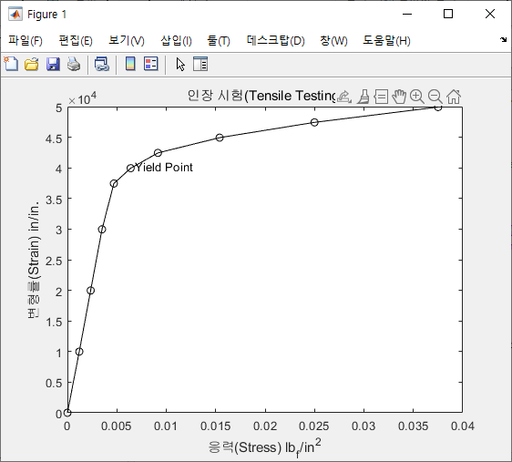
먼저 위의 Matlab 코드를 실행한 결과, 그에 해당하는 Plot을 보이면 다음과 같다.
그런데 다음의 전형적인 Structural Steel의 S-S 다이어그램과는 다르게
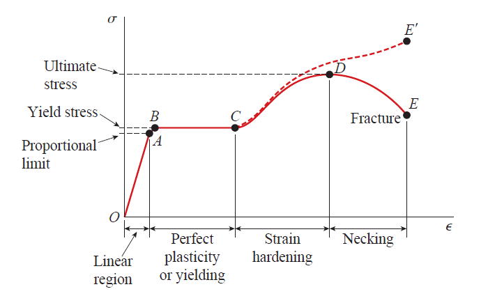
항복점을 결정하기가 쉽지 않은데, 이러한 경우에 James M. Gere의 Mechanics of Materials 책의 다음 내용에 의해,
When a material such as aluminum does not have an obvious yield point and yet undergoes large strains after the proportional limit is exceeded, an arbitrary yield stress may be determined by offset method.
이러한 경우 0.2% offset 방법을 이용할 수 있고, 이로부터 항복점을 도출해낼 수 있다.
이를 위해서는 우선 선형구간을 설정할 필요가 있는데, 육안으로 확인해보면 대략 Stress와 Strain의 앞의 4개의 데이터를 선형구간으로 설정할 수 있다.
이러한 경우 Stress와 Strain의 앞의 2개의 데이터만을 가지고 직선의 기울기를 도출하더라도 앞의 4개의 데이터 중 임의로 2개의 데이터를 택하여 직선의 기울기를 도출한 것과 동일하므로(선형구간이기 때문에), 편의를 위하여 다음과 같이 앞의 2개의 데이터만을 가지고 직선의 기울기를 도출한다.
D = 0.505;      % in.
A = pi/4*D*D;   % in.^{2}
F = [0:2000:6000,7500:500:10000];       % lb_{f}
L = [2.000, 2.0024, 2.0047, 2.0070, 2.0094, 2.0128, 2.0183, ...
    2.0308, 2.0500, 2.075];             % in.
Lz = L(1);      % in.

Stress = F./A;      % lb_{f}/in.^{2}
Strain = (L-Lz)/Lz;     % in./in. i.e. Dimensionless

plot(Strain, Stress, '-ok');
title('인장 시험(Tensile Testing)');
xlabel(strcat('응력(Stress)', texlabel(' lb_{f}/in.^{2}')));
ylabel(strcat('변형률(Strain)', texlabel(' in./in.')));

slope = (Stress(2) - Stress(1))/(Strain(2) - Strain(1));
그 다음, x에 대한 data sets들을 0.002에서부터 임의의 지점(직선이 위에서 plot한 S-S Diagram과 만날 수 있는 지점)까지 생성해주고, x에 대한 y의 data sets들도 생성해주자.
이때, y는 x축 방향으로 0.002만큼의 평행이동이 고려되어야 한다.
그 이유는 0.2% offset 방법이라는 것이 선형구간에서의 기울기를 가지는 직선을 0.2%만큼 평행이동하여 S-S Diagram과 만나는 점을 항복점으로 설정하는 방법이기 때문이다. 또한, 0.2% offset 방법의 이름에서처럼 0.2%를 사용해야 할 것으로 보이지만, 지금 현재 x축(Strain)은 % 단위가 아니고, Dimensionless 즉, 무차원이기 때문에 0.2%를 그대로 사용해서는 안되고 0.002로 해야한다.
그러므로 이러한 사항들을 고려하여 Matlab 코드를 작성하면 다음과 같다.
D = 0.505;      % in.
A = pi/4*D*D;   % in.^{2}
F = [0:2000:6000,7500:500:10000];       % lb_{f}
L = [2.000, 2.0024, 2.0047, 2.0070, 2.0094, 2.0128, 2.0183, ...
    2.0308, 2.0500, 2.075];             % in.
Lz = L(1);      % in.

Stress = F./A;      % lb_{f}/in.^{2}
Strain = (L-Lz)/Lz;     % in./in. i.e. Dimensionless

plot(Strain, Stress, '-ok');
title('인장 시험(Tensile Testing)');
xlabel(strcat('응력(Stress)', texlabel(' lb_{f}/in.^{2}')));
ylabel(strcat('변형률(Strain)', texlabel(' in./in.')));

slope = (Stress(2) - Stress(1))/(Strain(2) - Strain(1));
x = 0.002:.001:0.01;
y = slope * (x - 0.002);
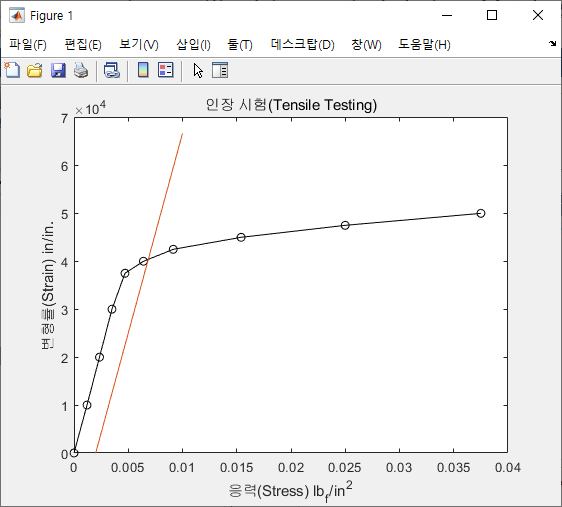
또한, 구성한 직선을 위에서 만든 S-S Diagram과 동시에 그리는 코드를 작성하면 다음과 같고,
D = 0.505;      % in.
A = pi/4*D*D;   % in.^{2}
F = [0:2000:6000,7500:500:10000];       % lb_{f}
L = [2.000, 2.0024, 2.0047, 2.0070, 2.0094, 2.0128, 2.0183, ...
    2.0308, 2.0500, 2.075];             % in.
Lz = L(1);      % in.

Stress = F./A;      % lb_{f}/in.^{2}
Strain = (L-Lz)/Lz;     % in./in. i.e. Dimensionless

plot(Strain, Stress, '-ok');
title('인장 시험(Tensile Testing)');
xlabel(strcat('응력(Stress)', texlabel(' lb_{f}/in.^{2}')));
ylabel(strcat('변형률(Strain)', texlabel(' in./in.')));

slope = (Stress(2) - Stress(1))/(Strain(2) - Strain(1));
x = 0.002:.001:0.01;
y = slope * (x - 0.002);

hold on;

plot(x, y);
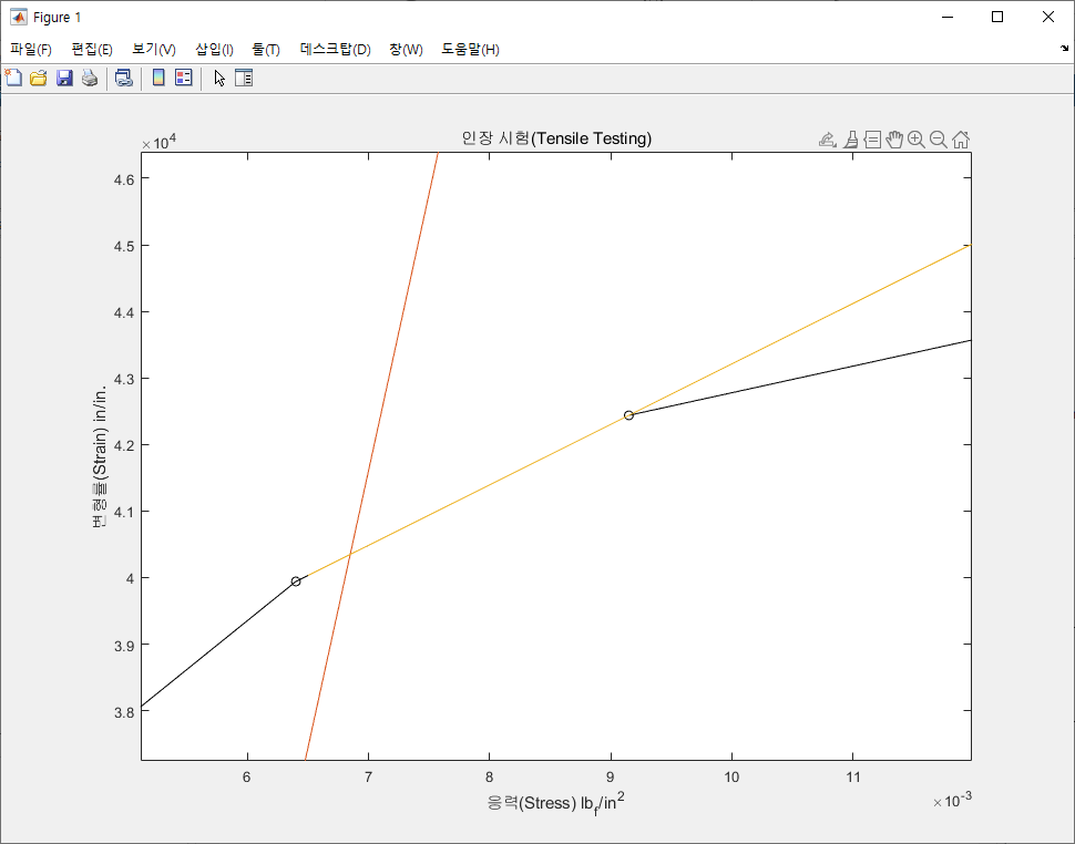
그 결과는 다음과 같다.
위에서 그린 Plot을 확대해보면, 직선과 S-S Diagram이 만나는 점이 다음에서 확인할 수 있는 것과 같이 S-S Diagram 위에 Circle Marker로 표시한 점과는 다른 점임을 확인할 수 있다.
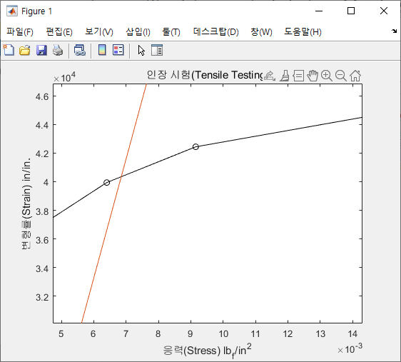
그러므로 S-S Diagram과 위에서 Plot한 직선이 만나는 Intersection Point를 찾기 위해서는 먼저 본 문제에 주어진 데이터들이 Discretized되어져 있다는 사실로부터 직선과 S-S Diagram이 만나는 곳의 S-S Diagram이 직선이라는 사실을 미루어 짐작해볼 수 있다.
그런데 지금 직선과 S-S Diagram이 교차하는 구간은 S-S Diagram의 6번째와 7번째 Data points들 사이의 구간이므로 두 Data points들에 대해서 위에서와 같이 직선의 관계를 형성해준다면, 직선과 S-S Diagram이 만나는 점을 찾는 것보다 직선과 직선이 만나는 점을 찾기가 훨씬 수월해진다.
이러한 사실로부터 해당 구간에 대한 직선 관계를 유도해내고 Plot하는 코드는 다음과 같다.
위에서 직선을 도출해낼 때 이미 그 과정을 보였으므로 자세한 과정은 생략한다.
D = 0.505;      % in.
A = pi/4*D*D;   % in.^{2}
F = [0:2000:6000,7500:500:10000];       % lb_{f}
L = [2.000, 2.0024, 2.0047, 2.0070, 2.0094, 2.0128, 2.0183, ...
    2.0308, 2.0500, 2.075];             % in.
Lz = L(1);      % in.

Stress = F./A;      % lb_{f}/in.^{2}
Strain = (L-Lz)/Lz;     % in./in. i.e. Dimensionless

plot(Strain, Stress, '-ok');
title('인장 시험(Tensile Testing)');
xlabel(strcat('응력(Stress)', texlabel(' lb_{f}/in.^{2}')));
ylabel(strcat('변형률(Strain)', texlabel(' in./in.')));

slope = (Stress(2) - Stress(1))/(Strain(2) - Strain(1));
x = 0.002:.001:0.01;
y = slope * (x - 0.002);

hold on;

plot(x, y);

slope_r = ((Stress(7)-Stress(6))/(Strain(7)-Strain(6)));
x1 = 0.0065:.001:0.0865;
y1 = slope_r*(x1-Strain(6))+Stress(6);

plot(x1, y1);
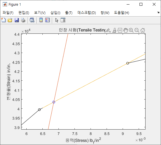
부연 설명하자면, 이 경우에는 위의 직선과는 다르게 y축 방향으로의 평행이동도 고려를 해주어야 다음에서와 같이 우리가 원하는 S-S Diagram과 직선이 만나는 구간에 대한 직선의 관계를 유도해낼 수 있다.
이제 Intersection Point를 찾아야 하는데, 위에서 두 직선의 관계를 x, y, x1, y1으로 유도했으므로 단순히 Matlab에서 제공해주는 polyxpoly Function을 사용해주면 된다.
그리고 해당 Intersection Point의 x좌표와 y좌표를 각각 Xz, Yz로 받고 이를 표시해주는 코드는 다음과 같다.
기존의 S-S Diagram에서 Circle Marker가 검은색이므로 이와의 구별을 위해서 파란색 Marker를 이용하였다.
D = 0.505;      % in.
A = pi/4*D*D;   % in.^{2}
F = [0:2000:6000,7500:500:10000];       % lb_{f}
L = [2.000, 2.0024, 2.0047, 2.0070, 2.0094, 2.0128, 2.0183, ...
    2.0308, 2.0500, 2.075];             % in.
Lz = L(1);      % in.

Stress = F./A;      % lb_{f}/in.^{2}
Strain = (L-Lz)/Lz;     % in./in. i.e. Dimensionless

plot(Strain, Stress, '-ok');
title('인장 시험(Tensile Testing)');
xlabel(strcat('응력(Stress)', texlabel(' lb_{f}/in.^{2}')));
ylabel(strcat('변형률(Strain)', texlabel(' in./in.')));

slope = (Stress(2) - Stress(1))/(Strain(2) - Strain(1));
x = 0.002:.001:0.01;
y = slope * (x - 0.002);

hold on;

plot(x, y);

slope_r = ((Stress(7)-Stress(6))/(Strain(7)-Strain(6)));
x1 = 0.0065:.001:0.0865;
y1 = slope_r*(x1-Strain(6))+Stress(6);

plot(x1, y1);

[Xz, Yz] = polyxpoly(x, y, x1, y1);

plot(Xz, Yz, '-ob');
그러면 다음과 같이 정확하게 Intersection Point를 도출해낼 수 있음을 확인할 수 있다.
지금까지 0.2% Offset Method에 의해서 해당 Intersection Point를 도출한 과정을 보였는데, 이는 문제에서 직접적으로 요구한 사항이 아니므로 이제 문제에서 요구한 Yield Point에 Text Box를 이용하여 표시해준다.
위의 섹션과 관련없는 plot 등과 같은 코드들은 삭제해준다.
코드를 보이면 다음과 같다.
이에 대한 결과를 보이면 다음과 같다.
댓글남기기