Mechanics of Materials: Tensile Strength Test - 3

Tensile Strength Test

지난 편에 이어서 재료역학 시간에 실시한 인장 시험 보고서의 내용을 공개하고자 한다.

다음으로 0.2% 오프셋에 의한 항복응력을 구하는 과정을 서술하겠다.

0.2% 오프셋에 의한 항복응력

먼저 항복응력에 대해서 설명하겠다.

물체에 힘을 가하여 양쪽으로 당긴다고 했을 때 그 물체의 길이는 어떻게 될까?

당연하게도 물체의 길이는 늘어나게 될 것이다.

그런데 여기서 어느 정도 힘을 가하고 그 힘을 놓게 된다면 그 물체는 다시 원래의 길이로 돌아가게 될 것이다.

하지만 일정 크기 이상의 힘으로 그 물체를 양쪽에서 당긴 후 힘을 놓게 된다면 그 물체는 원래 상태로 되돌아가지 못하고 더 길어지게 될 것이다.

이때, 물체에 인장력을 가하여 그 물체가 원래 상태로 돌아갈 수 있을 때의 최대 힘을 항복강도 또는 항복응력이라고 한다.

이러한 항복응력은 다음의 Stress-strain diagram에서 볼 수 있듯이 육안으로 확인할 수 있는 반면,

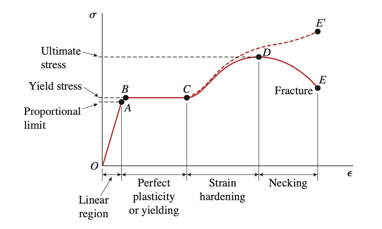
우리에게 주어진 데이터로부터 그려진 다음의 Stress-strain diagram의 경우에는

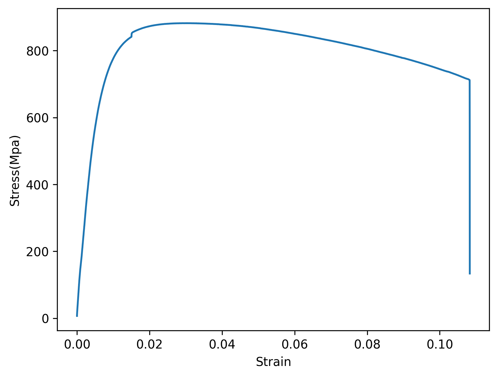
항복응력의 위치를 찾아내는 것이 어렵다.

그러므로 이러한 경우에 근사적으로 항복응력의 값을 도출하기 위해서 0.2% 오프셋 방법이 등장하게 되었다.

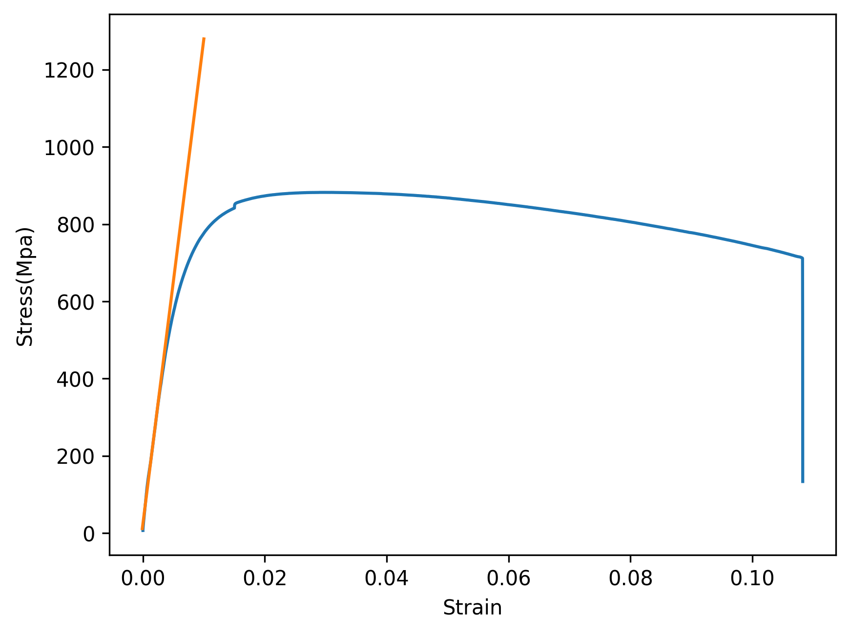
이 방법은 곡선의 초기 선형 구간에서의 직선을 0.2%(우리의 경우에는 기존 Elongation percent data를 100으로 나누었으므로 0.002)만큼 오른쪽으로 평행이동한 후 그 직선이 곡선과 만나는 지점의 Stress 값이 항복응력이 된다는 원리이다.

우리는 이전 시간에 탄성계수 즉, 곡선의 초기 선형 구간에서의 기울기를 도출했고 또 그때의 y절편도 도출했으므로 이 값들을 그대로 이용하여 일차함수를 구성해주고 Draw 한 후 직선과 곡선이 만나는 점의 y 좌표 값만 산출해주면 되겠다.

(일차함수보다 직선이 더 큰 개념이지만 실습 데이터로부터 그리고 0.2% 오프셋 방법으로부터 본 포스팅에서는 일차함수의 관점에서 서술하겠다.)

먼저 지난 시간에 작성한 코드를 가져오자.

import numpy as np
import matplotlib.pyplot as plt
import csv

sm = open("SM.csv", "r")
rdr = csv.reader(sm)
stress = []
strain = []
stress_ex = []
strain_ex = []

next(rdr); next(rdr)

for line in rdr:
    stress.append(float(line[8])); strain.append(float(line[9])/100)

for i in range(0, 350):
    stress_ex.append(stress[i])
    strain_ex.append(strain[i])

slope_intercept = np.polyfit(strain_ex, stress_ex, 1)

print(slope_intercept)

plt.plot(strain, stress)
plt.xlabel("Strain"); plt.ylabel("Stress(Mpa)")

plt.savefig("S-S Curve.png", dpi=300, bbox_inches="tight")

sm.close()

먼저 위 코드에서 slope_intercept를 출력하는 출력문을 삭제하자.

그 후, 직선을 Draw 하기 위해서 정의역에 대한 배열을 구성해주어야 하는데 numpy에서 linspace 함수를 제공해주므로 이를 이용하자.

import numpy as np
import matplotlib.pyplot as plt
import csv

sm = open("SM.csv", "r")
rdr = csv.reader(sm)
stress = []
strain = []
stress_ex = []
strain_ex = []

next(rdr); next(rdr)

for line in rdr:
    stress.append(float(line[8])); strain.append(float(line[9])/100)

for i in range(0, 350):
    stress_ex.append(stress[i])
    strain_ex.append(strain[i])

slope_intercept = np.polyfit(strain_ex, stress_ex, 1)

x = np.linspace(-0.0001, 0.01, 10000)           # -0.0001 ~ 0.01에서 10000개의 element를 가진 numpy array를 생성한다.

plt.plot(strain, stress)
plt.xlabel("Strain"); plt.ylabel("Stress(Mpa)")

plt.savefig("S-S Curve.png", dpi=300, bbox_inches="tight")

sm.close()

정의역을 구성했다면 이제 치역을 구성하자.

import numpy as np
import matplotlib.pyplot as plt
import csv

sm = open("SM.csv", "r")
rdr = csv.reader(sm)
stress = []
strain = []
stress_ex = []
strain_ex = []

next(rdr); next(rdr)

for line in rdr:
    stress.append(float(line[8])); strain.append(float(line[9])/100)

for i in range(0, 350):
    stress_ex.append(stress[i])
    strain_ex.append(strain[i])

slope_intercept = np.polyfit(strain_ex, stress_ex, 1)

x = np.linspace(-0.0001, 0.01, 10000)           
y = slope_intercept[0] * x + slope_intercept[1]             # slope_intercept의 첫 번째 데이터가 slope이고 두 번째 데이터가 y-intercept이다.

plt.plot(strain, stress)
plt.xlabel("Strain"); plt.ylabel("Stress(Mpa)")

plt.savefig("S-S Curve.png", dpi=300, bbox_inches="tight")

sm.close()

그 후 plot 함수의 추가 인자로 x와 y를 넘겨주자.

import numpy as np
import matplotlib.pyplot as plt
import csv

sm = open("SM.csv", "r")
rdr = csv.reader(sm)
stress = []
strain = []
stress_ex = []
strain_ex = []

next(rdr); next(rdr)

for line in rdr:
    stress.append(float(line[8])); strain.append(float(line[9])/100)

for i in range(0, 350):
    stress_ex.append(stress[i])
    strain_ex.append(strain[i])

slope_intercept = np.polyfit(strain_ex, stress_ex, 1)

x = np.linspace(-0.0001, 0.01, 10000)           
y = slope_intercept[0] * x + slope_intercept[1]             

plt.plot(strain, stress, x, y)              # plot 함수의 추가 인자로 x와 y를 넘겨줌.
plt.xlabel("Strain"); plt.ylabel("Stress(Mpa)")

plt.savefig("S-S Curve.png", dpi=300, bbox_inches="tight")

sm.close()

위 코드 실행 후 동일 Directory 내에 생성된 S-S Curve.png의 결과가 다음과 같다면 성공이다.

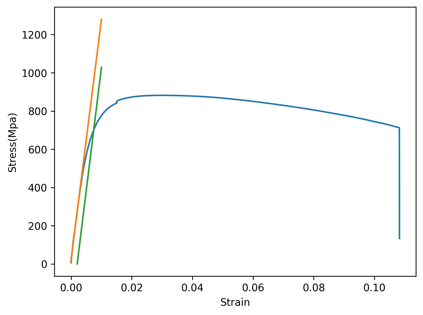
동일한 방식으로 직선을 하나 더 그려야하기 때문에 정의역을 하나 더 구성해주고, 그 때의 치역도 하나 더 구성해주자.

치역에 대한 식을 작성할 때는 위에서 설명했듯이 0.002만큼 오른쪽으로의 평행이동을 고려하고, 그래프가 깔끔하게 그려지도록 y 값이 0보다 크거나 같은 구간에서만 Draw가 되도록 하자.

즉, 치역에 y가 0보다 크거나 같다는 제한을 두면 된다.

import numpy as np
import matplotlib.pyplot as plt
import csv

sm = open("SM.csv", "r")
rdr = csv.reader(sm)
stress = []
strain = []
stress_ex = []
strain_ex = []

next(rdr); next(rdr)

for line in rdr:
    stress.append(float(line[8])); strain.append(float(line[9])/100)

for i in range(0, 350):
    stress_ex.append(stress[i])
    strain_ex.append(strain[i])

slope_intercept = np.polyfit(strain_ex, stress_ex, 1)

x = np.linspace(-0.0001, 0.01, 10000)           
x1 = np.linspace(0.002, 0.01, 8112)                # 0.002 ~ 0.01에서 8112개의 element를 가진 numpy array를 생성한다.
y = slope_intercept[0] * x + slope_intercept[1]             
y1 = list(filter(lambda y1: y1 >= 0, slope_intercept[0] * (x - 0.002) + slope_intercept[1]))      # 0.002만큼 오른쪽으로의 평행이동과 깔끔한 그래프 Draw를 위한 y1이 0보다 크거나 같다는 제한

plt.plot(strain, stress, x, y)
plt.xlabel("Strain"); plt.ylabel("Stress(Mpa)")

plt.savefig("S-S Curve.png", dpi=300, bbox_inches="tight")

sm.close()

그 다음, 다음과 같이 plot의 추가 인자로 x1과 y1을 보내주자.

import numpy as np
import matplotlib.pyplot as plt
import csv

sm = open("SM.csv", "r")
rdr = csv.reader(sm)
stress = []
strain = []
stress_ex = []
strain_ex = []

next(rdr); next(rdr)

for line in rdr:
    stress.append(float(line[8])); strain.append(float(line[9])/100)

for i in range(0, 350):
    stress_ex.append(stress[i])
    strain_ex.append(strain[i])

slope_intercept = np.polyfit(strain_ex, stress_ex, 1)

x = np.linspace(-0.0001, 0.01, 10000)           
x1 = np.linspace(0.002, 0.01, 8112)                
y = slope_intercept[0] * x + slope_intercept[1]             
y1 = list(filter(lambda y1: y1 >= 0, slope_intercept[0] * (x - 0.002) + slope_intercept[1]))      

plt.plot(strain, stress, x, y, x1, y1)              # plot 함수의 추가 인자로 x1과 y1을 인자로 보내줌.
plt.xlabel("Strain"); plt.ylabel("Stress(Mpa)")

plt.savefig("S-S Curve.png", dpi=300, bbox_inches="tight")

sm.close()

위 코드 실행 후 S-S Curve.png의 결과가 다음과 같다면 성공이다.

마지막으로 평행이동한 직선과 곡선이 만나는 점의 y 좌표를 산출해야 하는데, 필자는 이것을 위한 별도의 알고리즘 구현없이 shapely라는 패키지를 이용하여 처리하였다.

shapely는 직교 좌표 평면에서의 geometric objects들에 대한 조작 및 분석과 관련된 기능들을 제공해주는 패키지이다.

먼저 다음과 같이 평행이동한 직선에 대해서 LineString 클래스에 대한 객체를 생성하고, 마찬가지로 S-S Curve에 대해서도 LineString 클래스에 대한 객체를 생성하자.

import numpy as np
import matplotlib.pyplot as plt
import csv
from shapely.geometry import LineString

sm = open("SM.csv", "r")
rdr = csv.reader(sm)
stress = []
strain = []
stress_ex = []
strain_ex = []

next(rdr); next(rdr)

for line in rdr:
    stress.append(float(line[8])); strain.append(float(line[9])/100)

for i in range(0, 350):
    stress_ex.append(stress[i])
    strain_ex.append(strain[i])

slope_intercept = np.polyfit(strain_ex, stress_ex, 1)

x = np.linspace(-0.0001, 0.01, 10000)           
x1 = np.linspace(0.002, 0.01, 8112)                
y = slope_intercept[0] * x + slope_intercept[1]             
y1 = list(filter(lambda y1: y1 >= 0, slope_intercept[0] * (x - 0.002) + slope_intercept[1]))      

line_1 = LineString(np.column_stack((x1, y1)))          # 평행이동한 직선에 대한 LineString 객체 생성
line_2 = LineString(np.column_stack((strain, stress)))          # S-S Curve에 대한 LineString 객체 생성

plt.plot(strain, stress, x, y, x1, y1)
plt.xlabel("Strain"); plt.ylabel("Stress(Mpa)")

plt.savefig("S-S Curve.png", dpi=300, bbox_inches="tight")

sm.close()

그 후 평행이동한 직선과 S-S Curve의 교차점을 찾기 위해 intersection 함수를 이용하자.

import numpy as np
import matplotlib.pyplot as plt
import csv
from shapely.geometry import LineString

sm = open("SM.csv", "r")
rdr = csv.reader(sm)
stress = []
strain = []
stress_ex = []
strain_ex = []

next(rdr); next(rdr)

for line in rdr:
    stress.append(float(line[8])); strain.append(float(line[9])/100)

for i in range(0, 350):
    stress_ex.append(stress[i])
    strain_ex.append(strain[i])

slope_intercept = np.polyfit(strain_ex, stress_ex, 1)

x = np.linspace(-0.0001, 0.01, 10000)           
x1 = np.linspace(0.002, 0.01, 8112)                
y = slope_intercept[0] * x + slope_intercept[1]             
y1 = list(filter(lambda y1: y1 >= 0, slope_intercept[0] * (x - 0.002) + slope_intercept[1]))      

line_1 = LineString(np.column_stack((x1, y1)))          
line_2 = LineString(np.column_stack((strain, stress)))          

intersection = line_1.intersection(line_2)          # line_1과 line_2의 교차점에 대한 representation을 intersection에 저장

plt.plot(strain, stress, x, y, x1, y1)
plt.xlabel("Strain"); plt.ylabel("Stress(Mpa)")

plt.savefig("S-S Curve.png", dpi=300, bbox_inches="tight")

sm.close()

그 다음, x와 y 좌표를 각각 x_c와 y_c에 삽입하자.

import numpy as np
import matplotlib.pyplot as plt
import csv
from shapely.geometry import LineString

sm = open("SM.csv", "r")
rdr = csv.reader(sm)
stress = []
strain = []
stress_ex = []
strain_ex = []

next(rdr); next(rdr)

for line in rdr:
    stress.append(float(line[8])); strain.append(float(line[9])/100)

for i in range(0, 350):
    stress_ex.append(stress[i])
    strain_ex.append(strain[i])

slope_intercept = np.polyfit(strain_ex, stress_ex, 1)

x = np.linspace(-0.0001, 0.01, 10000)           
x1 = np.linspace(0.002, 0.01, 8112)                
y = slope_intercept[0] * x + slope_intercept[1]             
y1 = list(filter(lambda y1: y1 >= 0, slope_intercept[0] * (x - 0.002) + slope_intercept[1]))      

line_1 = LineString(np.column_stack((x1, y1)))          
line_2 = LineString(np.column_stack((strain, stress)))    

intersection = line_1.intersection(line_2)          
x_c, y_c = intersection.xy          # x와 y 좌표를 각각 x_c와 y_c에 삽입

plt.plot(strain, stress, x, y, x1, y1)
plt.xlabel("Strain"); plt.ylabel("Stress(Mpa)")

plt.savefig("S-S Curve.png", dpi=300, bbox_inches="tight")

sm.close()

마지막으로 교차점을 그래프에 표시하고, 교차점의 x좌표와 y좌표를 출력하자.

import numpy as np
import matplotlib.pyplot as plt
import csv
from shapely.geometry import LineString

sm = open("SM.csv", "r")
rdr = csv.reader(sm)
stress = []
strain = []
stress_ex = []
strain_ex = []

next(rdr); next(rdr)

for line in rdr:
    stress.append(float(line[8])); strain.append(float(line[9])/100)

for i in range(0, 350):
    stress_ex.append(stress[i])
    strain_ex.append(strain[i])

slope_intercept = np.polyfit(strain_ex, stress_ex, 1)

x = np.linspace(-0.0001, 0.01, 10000)           
x1 = np.linspace(0.002, 0.01, 8112)                
y = slope_intercept[0] * x + slope_intercept[1]             
y1 = list(filter(lambda y1: y1 >= 0, slope_intercept[0] * (x - 0.002) + slope_intercept[1]))      

line_1 = LineString(np.column_stack((x1, y1)))          
line_2 = LineString(np.column_stack((strain, stress)))    

intersection = line_1.intersection(line_2)          
x_c, y_c = intersection.xy         

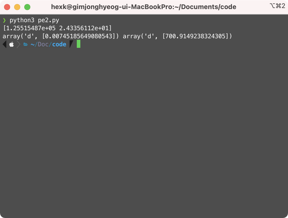
print(x_c, y_c)             # 교차점의 x좌표와 y좌표 출력

plt.plot(strain, stress, x, y, x1, y1)
plt.plot(*intersection.xy, 'ro')            # 그래프에 교차점 표시
plt.xlabel("Strain"); plt.ylabel("Stress(Mpa)")

plt.savefig("S-S Curve.png", dpi=300, bbox_inches="tight")

sm.close()

x와 y좌표가 각각 다음과 같이 출력되고,

그래프에 교차점이 다음과 같이 표시된다면 성공이다.

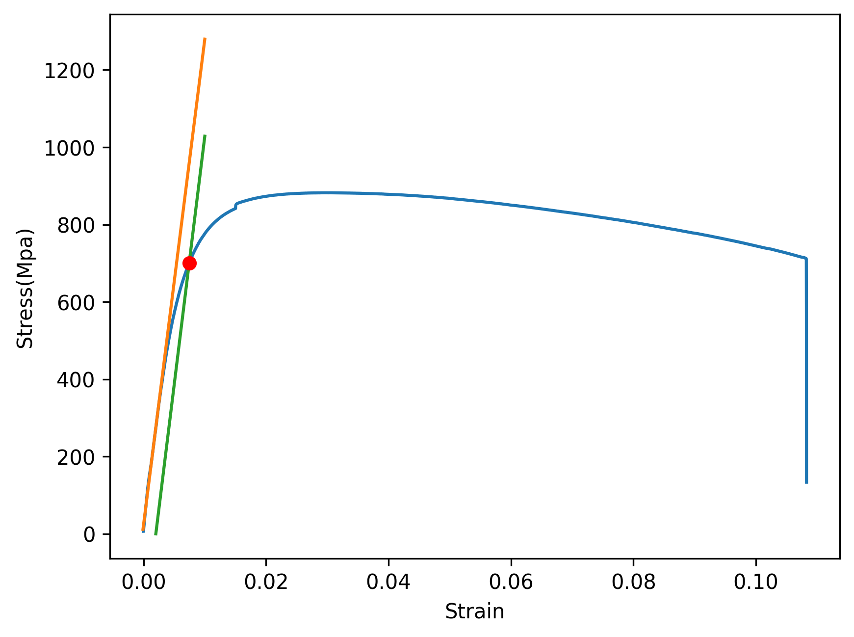
결론적으로 항복응력은 대략 700 근처임을 유추할 수 있겠다.

여기까지 이번 포스팅을 마무리 짓고 다음 포스팅에서는 극한강도와 파단연신율을 산출했던 과정을 설명하도록 하겠다.